Solutions

Frameworks

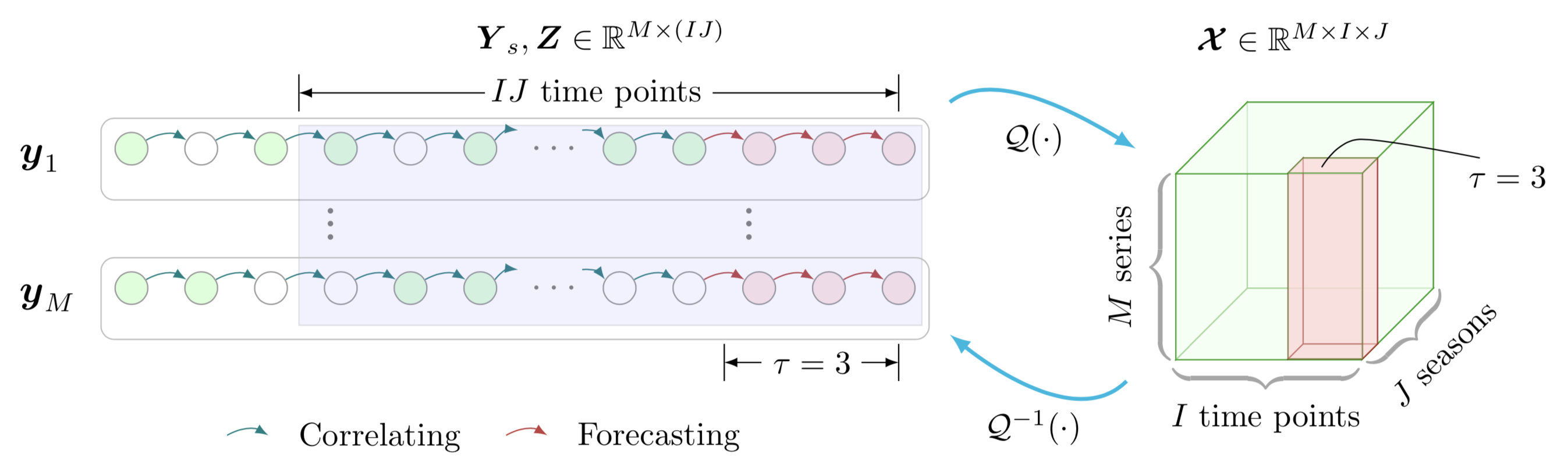
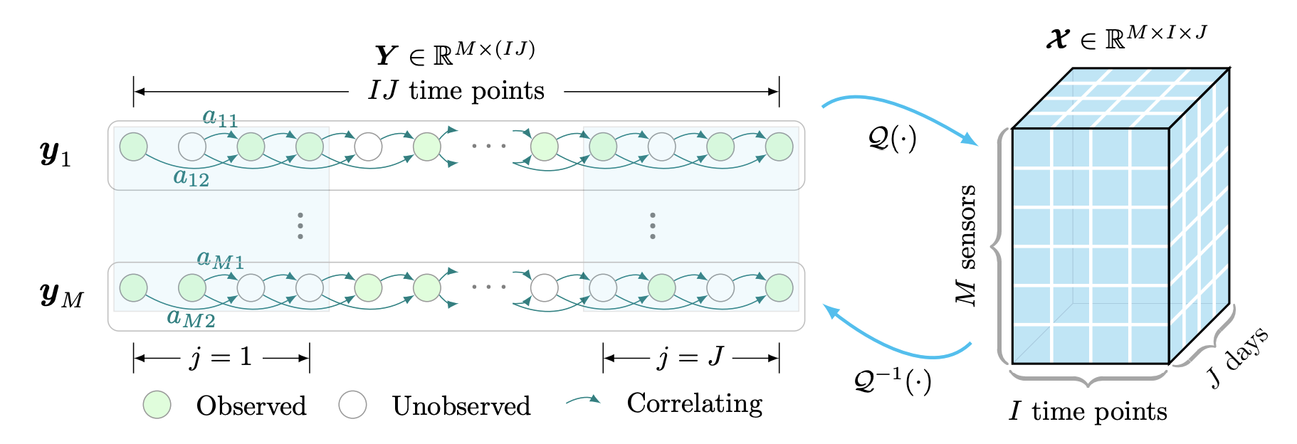
• Low-rank autoregressive tensor completion for multivariate time series prediction:

Algorithms

In what follows, we provide some simple time series imputation and forecasting approaches with Python implementation.

• Multivariate time series imputation
  • Low-rank autoregressive tensor completion
• Multivariate time series forecasting
  • VAR with ordinary least squares (OLS)
  • VAR with reduced-rank regression (RRR)

Low-rank autoregressive tensor completion

The low-rank autoregressive tensor completion model includes two important components, i.e., truncated nuclear norm and time series autoregression:

Below is the Python implementation.

import numpy as np

def ten2mat(tensor, mode):
    """mode = 0,1,2 refer to the mode-1, mode-2, and mode-3 unfoldings, respectively."""
    return np.reshape(np.moveaxis(tensor, mode, 0), (tensor.shape[mode], -1), order = 'F')

def mat2ten(mat, dim, mode):
    index = list()
    index.append(mode)
    for i in range(dim.shape[0]):
        if i != mode:
            index.append(i)
    return np.moveaxis(np.reshape(mat, list(dim[index]), order = 'F'), 0, mode)

def svt_tnn(mat, tau, theta):
    """Singular value thresholding algorithm for truncated nuclear norm minimization."""
    [m, n] = mat.shape
    if 2 * m < n:
        u, s, v = np.linalg.svd(mat @ mat.T, full_matrices = 0)
        s = np.sqrt(s)
        idx = np.sum(s > tau)
        mid = np.zeros(idx)
        mid[: theta] = 1
        mid[theta : idx] = (s[theta : idx] - tau) / s[theta : idx]
        return (u[:, : idx] @ np.diag(mid)) @ (u[:, : idx].T @ mat)
    elif m > 2 * n:
        return svt_tnn(mat.T, tau, theta).T
    u, s, v = np.linalg.svd(mat, full_matrices = 0)
    idx = np.sum(s > tau)
    vec = s[: idx].copy()
    vec[theta : idx] = s[theta : idx] - tau
    return u[:, : idx] @ np.diag(vec) @ v[: idx, :]

def compute_mape(var, var_hat):
    return np.sum(np.abs(var - var_hat) / var) / var.shape[0]

def compute_rmse(var, var_hat):
    return  np.sqrt(np.sum((var - var_hat) ** 2) / var.shape[0])

from scipy import sparse

def generate_Psi(dim_time, time_lags):
    Psis = []
    d = np.max(time_lags)
    for i in range(len(time_lags) + 1):
        row = np.arange(0, dim_time - d)
        if i == 0:
            col = np.arange(0, dim_time - d) + d
        else:
            col = np.arange(0, dim_time - d) + d - time_lags[i - 1]
        data = np.ones(dim_time - d)
        Psi = sparse.coo_matrix((data, (row, col)), shape = (dim_time - d, T))
        Psis.append(Psi)
    return Psis

from scipy.sparse.linalg import spsolve as spsolve

VAR with ordinary least squares (OLS)

For the vector autoregressive (VAR) model:

Then, the ordinary least squares (OLS) solution is given by

where is required to be non-singular (invertible).

Below is the VAR-OLS algorithm reproduced by using Python.

import numpy as np

def var_ols(X, d):
    N, T = X.shape
    Y = X[:, d : T]
    Z = np.zeros((d * N, T - d))
    for k in range(d):
        Z[k * N : (k + 1) * N, :] = X[:, d - (k + 1) : T - (k + 1)]
    A = Y @ np.linalg.pinv(Z)
    return A

VAR with reduced-rank regression (RRR)

The reduced-rank regression solution to the reduced-rank VAR model is given by

where consists of the eigenvectors corresponding to the largest eigenvalues of the matrix .

Below is the VAR-RRR algorithm reproduced by using Python.

import numpy as np

def var_rrr(X, d, R):
    N, T = X.shape
    Y = X[:, d : T]
    Z = np.zeros((d * N, T - d))
    for k in range(d):
        Z[k * N : (k + 1) * N, :] = X[:, d - (k + 1) : T - (k + 1)]
    A_ols = Y @ np.linalg.pinv(Z)
    u, _, _ = np.linalg.svd(A_ols @ Z, full_matrices = 0)
    Phi = u[:, : R]
    A = Phi @ Phi.T @ A_ols
    return A

If we have the coefficient matrix trained on the multivariate time series data , then we can perfrom forecasting on the test data with a certain time horizon. Note that the time horizons are the time steps that should be forecasted on the test data.

import numpy as np

def var_forecast(X_new, A, d, time_horizon):
    N, T = X_new.shape
    mat = np.append(X_new, np.zeros((N, time_horizon)), axis = 1)
    for t in range(time_horizon):
        mat[:, T + t] = A @ mat[:, T + t - np.arange(1, d + 1)].T.reshape(d * N)
    return mat[:, - time_horizon :]

Nonstationary time series data

Given the multivariate time series data consisting of (nonstationary), the differenced time series is the change between consecutive observations in the original time series, and can be written as

The constructed time series is the first-order differencing, usually appears to be stationary [Stationarity and differencing].

def first_diff(X):
    X_tilde = X[:, 1 :] - X[:, : -1]
    return X_tilde